Algos Expeditus

In order to get into the workings behind a neural network, let's build up from the concepts of logistic regression. Remember this flow chart from logistic regression? This, Logistic regression,  can be visualized as a very basic neural network :  Where one neuron computes z and then applies the  $ Z = w^TX+b $ and then applies a non-linear activation function $ A = g(Z)$ (where $g(z) = \sigma(z)$ in this case) A neural network is basically a logistic regression on steroids! This is what a typical neural network looks like :  It contains 3 layers; The input layer, The hidden layer(s), and The output layer. In a neural network, the input layer contains the values x, and the output layer contains the predicted value of y. The layers in between are called "hidden layers" because the true value of these nodes are not observed.   Each neuron in a neural network does the exact same thing here as well (calculates $ Z = w^TX+b $ and then applies a non-linear activation function $

NumPy is a python library used for applying high-level mathematical functions to multi-dimensional arrays and matrices. In our case it would help us in vectorization. Vectorization refers to the solution which allow the application of operations to an entire set of arrays at once instead of applying it one element at a time (as is done in case of loops) Vectorization is much much faster than the traditional loops and most computer can do it more efficiently ( Here is a sample of code to demonstrate just how fast it is) But before we start with matrices and vectorization and broadcasting and what not, let's start with the very basics and learn how to make and modify matrices NumPy is usually enabled by default, nevertheless. You can check check it from the Anaconda Navigator   (if you don't know about Anaconda Navigator and don't know how to install packages, check the following link ) Now, Open Jupyter notebooks, go to whatever folder you want to save the file in and let&#

Computational Graph is a directional graph where each nodes is associated with some mathematical operation. We'll use these computational graph to understand we find the partial derivates of Cost Function with respect to different weights and biases To understand how to calculate the partial derivatives through a computational graph, let's assume for a second that J is a function of 3 parameters, a, b and c. And that J is expressed as $$J = 3(a+bc)$$ When thinking about how to step-by-step compute J, you'll realize that you'll have to first calculate b*c , let us that product is u .  We then have to add this u with a . Let us now call this sum v . And finally, we'll have to multiply this v with 3, in order to (finally) get J . Let's visualize this with our computational graph   Let's assign some random values to a, b, and c. Now, we know, that by it's very definition, the derivative of a funciton x with respect to y tells us the rate of change of x wit

Recall that Cost Function (J),  is a function of our parameters w(weights), and b(bias)...and that cost function tells us how bad we are doing. So, in order to reduce our cost function, it's only logical to tweak our weights and bias. Here's a picture that illustrates various costs with respect to different weights and biases (here, for the sake of simplicity, we assume that cost function is a function of only 1 weight and 1 bias) Image source :  https://suniljangirblog.wordpress.com/2018/12/03/the-outline-of-gradient-descent/ Here, x represents the weights, y represents the bias and z represents the Cost As we can see, our aim through Gradient Descent is to reach lowest Cost, i.e., the lowest point in the z-axis that lies in the convex plane. This lowest part of the curve/plane is what we call as the "minimum of the graph". And if you're acquainted with basic calculus, you'd know that there are two types of minima; the local minima and the absolute minima. We

INTRO Logistic Regression is a learning algorithm used for classification, i.e., given an input feature vector x, the output y will be some discrete value, i.e., either 0 or 1 (representing no or yes in a binary classification) or 0, 1, 2..and so on (if we're classifying between multiple categories say, cat, dog, trees etc) Given an input feature vector x, corresponding to an image that you want to classify as either cat (y = 1), or not cat (y = 0), we want the algorithm to output a prediction ($\hat y$) that is an estimate of y, i.e., the probability of it being y (probability of it being a cat) If x is an n x dimensional vector. Given that information, the parameters of logistic regression would be:  w, which is also an n x  dimensional vector b, which is just a real number Given the input x and the parameters w and b, this prediction could be generated as   $$ \hat y= \sigma (w^Tx+b) $$   Where $ \sigma (w^Tx+b) $ is $$  \sigma(

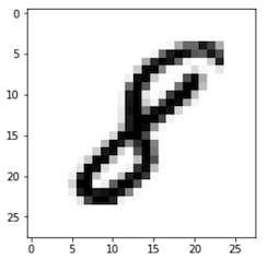
Before we dive right into the various algorithms of deep learning, we should get acquainted with the common notations used. Consider this image of a digit Image source : MNIST This training example contains a 28x28 pixel image along with its correct label, i.e, 8. Within the computer, this image is stored as a matrix of pixel intensities Each pixel contains within it, a number from 0-255 representing the intensity of black (with 0 being total absence of black, i.e., white, and 255 being totally black) Therefore, in the eyes of a computer, this image would be something like this  If we try to turn these pixel intensity values into a feature vector, what we do is unroll all these pixel intensity values into an input feature vector x. So we'll take all the pixel values starting from 0, 0, 0....1, 12, 0, 11, 39... until we get a very long feature vector (of size (64x64 =)4096) listing out all the pixel intensities $$X = \begin{bmatrix} 0 \\ 0 \\ . \\ . \\ . \\ 1 \\ 12 \\ 0 \\ 11 \\ . \

Image source :  https://www.anaconda.com/ OK. First Off, Intro (What Anaconda? Why Anaconda? How Anaconda?) Paraphrasing from Wikipedia ( https://en.wikipedia.org/wiki/Anaconda_(Python_distribution) ): Anaconda is a free and open-source distribution of Python that serves as the perfect platform for scientific computing, Data Analysis, Machine Learning (our main interest) Anaconda makes is really simple to apply machine learning projects, and is really great at managing packages. To install Anaconda  Go to  https://www.anaconda.com/products/individual Scroll waaaayyyy down, until you see something like this : Download the appropriate package (according to your computer OS and architecture). Also, Make sure you're downloading for Python 3.7 During the installation, don't forget to check the following options when prompted: After you're done with  the installation, there's another small thing I want you to introduce... Environments And here we come to the main reason we